Utilities

>> awcgen --help

Usage: awcgen [input file] [output file] [flags]

  Flags:  t  'Test mode'    Produce two-column output for easy plotting.
          m  'More points'  Attempt to use ~16000 points instead of ~1600.
          f  'Full scale'   Produce a full-size waveform when driving a 50 Ohm load.

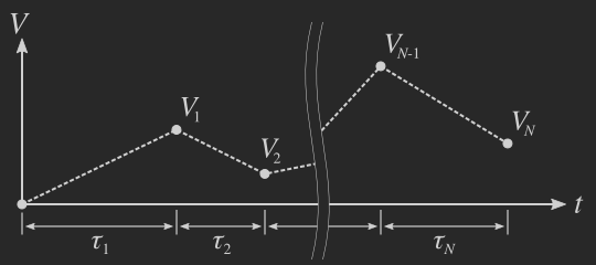
The input file should be a list of time periods τ_i (in seconds) and target voltages V_i (in Volts), separated by whitespace, one line per point. awcgen sets the initial value to 0 V, then ramps linearly to each V_i over τ_i in succession, as illustrated below. Abrupt jumps can be made by setting τ_i = 0.

In preparing the waveform, awcgen attempts to choose a sample rate that meets three goals (in order of importance):

1. Satisfies: f_samp = (40 MHz) / N where 1 ≤ N ≤ 2³⁴ - 1
2. Produces about 1600 points (to reduce transfer time).
3. Is a round number.

Complex waveforms, particularly those containing both large and small τ_i, may require more points to be faithfully reproduced. Supplying the 'm' flag will max out the number points available at the cost of a much longer transfer time. The output will be an AWC-compatible text file containing several lines of header information followed by a list of voltages V_j at times t_j = {0, t_samp, 2 t_samp, ...} where t_samp = 1 / f_samp.

>> awcgen example_pwl.txt example_awc.txt

             Request       Actual
             ------------  ------------
Divider:     13750.000     15625
Frequency:   2.909e+03     2.560e+03
N_points:    1600          1409

Total time:  5.500e-01
Output:      AWC-compatible

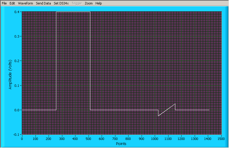
The output file can then be opened in AWC, and would look like this. If you do not have AWC handy or wish to verify the output as a continuous function V(t) rather than V_j, use the 't' flag:

>> awcgen example_pwl.txt example_test.txt t
...
Output:      Plot-compatible

This output file can then be easily loaded by plotting software, such as matplotlib.

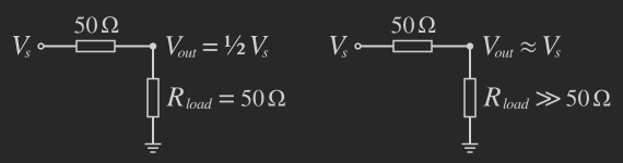
Notice that the amplitude in the previous example appears to be half that requested. The reason is related to the expected load impedance: The instrument provides a 50 Ω output, and expects a 50 Ω load, so it scales the internal source voltage V_s to produce the expected output V_out in that situation (below, left). In contrast, awcgen was written with a high-impedance load in mind (below, right), so by default it divides all voltages by two to counteract the above assumption. If you do plan to drive a 50 Ω load, simply supply the 'f' flag as mentioned in the usage.

>> npgsfixer --help

Usage: npgsfixer [input file] [output file] [arguments]

  Arguments:  --fieldbase [file]  Specify base filename of sub-fields, if applicable. Default: "field"
              --runfile   [file]  Specify filename of runfile snippet, if applicable. Default: "runfile.txt"

The input file should be a DesignCAD file containing the color-coded elements that make up your pattern. Filled shapes should be closed polylines of one of six colors (to accommodate dose ranges): light blue, medium blue, dark blue, light green, medium green, and dark green. (The exact RGB values for these colors can be found in the script.)

npgsfixer has two modes:

• Normal mode sets the appropriate flags on the elements in the pattern according to the color codes mentioned above. Unmatched elements are simply passed through unchanged.
• Fracture mode is automatically activated when at least one layer containing a yellow bounding box is detected. The pattern is fractured into separate files, one per bounding-boxed layer. Coordinates are adjusted to place the origin of each sub-field in the center of its bounding box.

Note: The same translation as in normal mode occurs in fracture mode and un-boxed layers are simply written to the main output file.

>> npgsfixer example_normal_in.DC2 example_normal_out.DC2
...
FIRST PASS:
...
SECOND PASS:
Processing layer 1 "0":
  Fixed filled polyline. Vertices: 4 Color: (0,0,255)
  Skipped non-filled polyline. Vertices: 12 Color: (255,0,0)
...
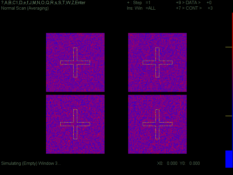
Processing layer 5 "write":
  Fixed filled polyline. Vertices: 12 Color: (0,0,255)
  Fixed filled polyline. Vertices: 12 Color: (0,0,255)
  Fixed filled polyline. Vertices: 20 Color: (0,0,255)
  Fixed filled polyline. Vertices: 63 Color: (0,0,255)
...
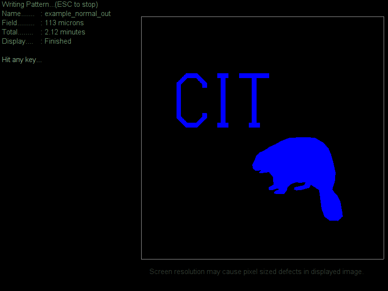
(See the full output here.)

The input file was created by importing a DXF file containing the pattern shown at right into DesignCAD. The output file example_normal_out.DC2 can then be loaded into NPGS via a runfile. In this case, the runfile does manual alignment using layers 1-4 (see screenshot) before writing layer 5 (see screenshot) to the sample.

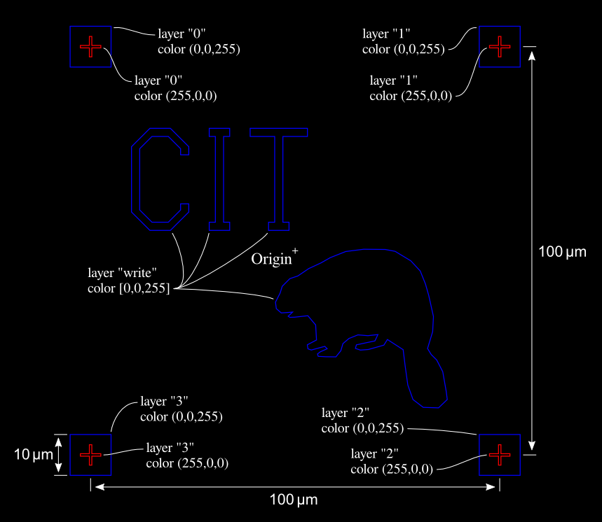
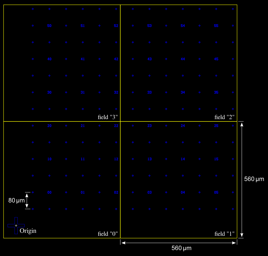
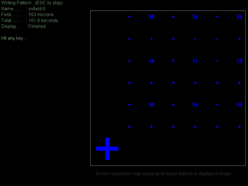
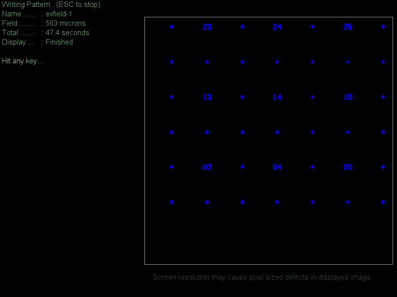
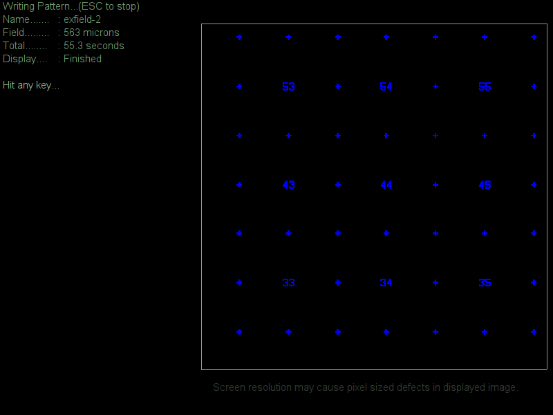
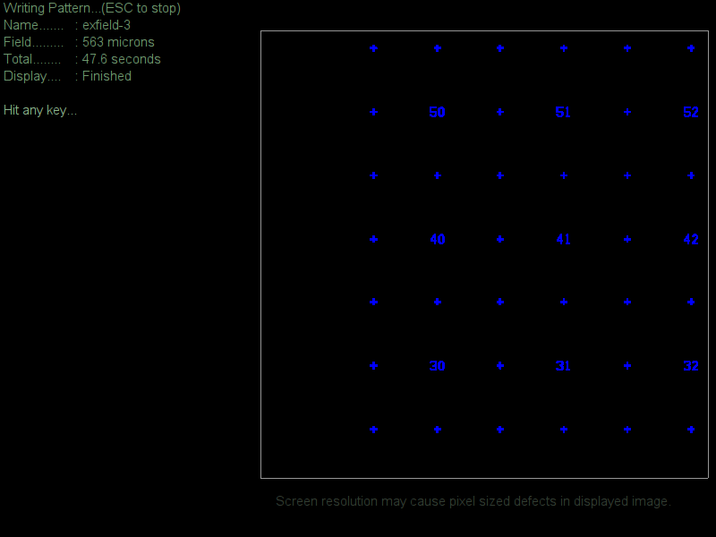
The test pattern (below, right) is a sparse alignment grid we want to write at higher magnification to get sharp features. npgsfixer will detect the yellow bounding boxes and fracture the pattern for us, generating a list of X-Y stage moves to stitch it back together during writing.

>> npgsfixer example_fracture_in.DC2 example_fracture_out.DC2 \
--fieldbase exfield --runfile exrun.txt
...
FIRST PASS:
Scanning layer 1 "0":
  Found bounding box. Vertices: 4, Center: (220.0, 220.0)
Scanning layer 2 "1":
  Found bounding box. Vertices: 4, Center: (780.0, 220.0)
Scanning layer 3 "2":
  Found bounding box. Vertices: 4, Center: (780.0, 780.0)
Scanning layer 4 "3":
  Found bounding box. Vertices: 4, Center: (220.0, 780.0)
SECOND PASS:
Processing layer 1 "0":
  Fixed filled polyline. Vertices: 12 Color: (0,0,255)
  Fixed filled polyline. Vertices: 12 Color: (0,0,255)
  ...
  Deleted bounding box.
...
(See the full output here.)

The input file was created by importing the original DXF file into DesignCAD. Given that all four layers include bounding boxes, the "main" output file contains no shapes and can be discarded. The fracture sub-fields were written to files exfield-{0,1,2,3}.DC2 and stage moves saved as a runfile snippet exrun.txt. A full-fledged runfile was then manually created based on the snippet, which writes the grid according to the scheme below:

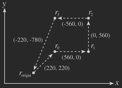
The four fields are written in order at locations {r₀, r₁, r₂, r₃} (see screenshots: "0", "1", "2", "3").